


Marco Molari
@mmolari.bsky.social
PostDoc @ Biozentrum - Basel in the group of Richard Neher
Interested in microbial genomics, pangenome graphs & evolution 🧬🦠💻
Interested in microbial genomics, pangenome graphs & evolution 🧬🦠💻
Thank you Will! 🙏 Coming from you who know the tool means a lot. Always inspiring to see it used!
January 7, 2025 at 12:59 PM
Thank you Will! 🙏 Coming from you who know the tool means a lot. Always inspiring to see it used!
Thank you so much! 🙏 Very very honored!
January 7, 2025 at 12:42 PM
Thank you so much! 🙏 Very very honored!
Thank you! 🙏 That’s so nice to hear!
January 6, 2025 at 8:53 PM
Thank you! 🙏 That’s so nice to hear!
[20/N]
We are curious to check in follow-up works whether these rates and patterns are specific to ST131, or are more general and can be found in other sequence types or even microbial species.
Hope you'll find the work interesting! Let us know if you have any observations or comments!
We are curious to check in follow-up works whether these rates and patterns are specific to ST131, or are more general and can be found in other sequence types or even microbial species.
Hope you'll find the work interesting! Let us know if you have any observations or comments!
January 6, 2025 at 5:12 PM
[20/N]
We are curious to check in follow-up works whether these rates and patterns are specific to ST131, or are more general and can be found in other sequence types or even microbial species.
Hope you'll find the work interesting! Let us know if you have any observations or comments!
We are curious to check in follow-up works whether these rates and patterns are specific to ST131, or are more general and can be found in other sequence types or even microbial species.
Hope you'll find the work interesting! Let us know if you have any observations or comments!
[19/N]
To explain the total structural diversity of the dataset, more than 2000 distinct structural variations must have happened in its short evolutionary history, corresponding to an average rate of one every 3 mutations on the core-genome. This is a remarkably high rate!
To explain the total structural diversity of the dataset, more than 2000 distinct structural variations must have happened in its short evolutionary history, corresponding to an average rate of one every 3 mutations on the core-genome. This is a remarkably high rate!
January 6, 2025 at 5:12 PM
[19/N]
To explain the total structural diversity of the dataset, more than 2000 distinct structural variations must have happened in its short evolutionary history, corresponding to an average rate of one every 3 mutations on the core-genome. This is a remarkably high rate!
To explain the total structural diversity of the dataset, more than 2000 distinct structural variations must have happened in its short evolutionary history, corresponding to an average rate of one every 3 mutations on the core-genome. This is a remarkably high rate!
[18/N]
Most of the IS integrations disrupt genes, and such structural gains would be interpreted as loss events in gene-based analyses. However, this happens less than expected by chance, indicating that roughly 2/3 of these integrations have already been removed by purifying selection.
Most of the IS integrations disrupt genes, and such structural gains would be interpreted as loss events in gene-based analyses. However, this happens less than expected by chance, indicating that roughly 2/3 of these integrations have already been removed by purifying selection.
January 6, 2025 at 5:12 PM
[18/N]
Most of the IS integrations disrupt genes, and such structural gains would be interpreted as loss events in gene-based analyses. However, this happens less than expected by chance, indicating that roughly 2/3 of these integrations have already been removed by purifying selection.
Most of the IS integrations disrupt genes, and such structural gains would be interpreted as loss events in gene-based analyses. However, this happens less than expected by chance, indicating that roughly 2/3 of these integrations have already been removed by purifying selection.
[17/N]
In binary junctions the vast majority of events are gains, often corresponding to an insertion sequence (IS) or prophage integrating in an otherwise conserved region of the genome. This corresponds to a rough rate of one of these events every 20 mutations on the core-genome.
In binary junctions the vast majority of events are gains, often corresponding to an insertion sequence (IS) or prophage integrating in an otherwise conserved region of the genome. This corresponds to a rough rate of one of these events every 20 mutations on the core-genome.

January 6, 2025 at 5:12 PM
[17/N]
In binary junctions the vast majority of events are gains, often corresponding to an insertion sequence (IS) or prophage integrating in an otherwise conserved region of the genome. This corresponds to a rough rate of one of these events every 20 mutations on the core-genome.
In binary junctions the vast majority of events are gains, often corresponding to an insertion sequence (IS) or prophage integrating in an otherwise conserved region of the genome. This corresponds to a rough rate of one of these events every 20 mutations on the core-genome.
[16/N]
For binary junctions we can go even further: they can be associated with gain or loss events.
In particular singleton junctions correspond to events on terminal branches of the tree, while non-singleton junctions can in principle be associated also to events on internal branches.
For binary junctions we can go even further: they can be associated with gain or loss events.
In particular singleton junctions correspond to events on terminal branches of the tree, while non-singleton junctions can in principle be associated also to events on internal branches.

January 6, 2025 at 5:12 PM
[16/N]
For binary junctions we can go even further: they can be associated with gain or loss events.
In particular singleton junctions correspond to events on terminal branches of the tree, while non-singleton junctions can in principle be associated also to events on internal branches.
For binary junctions we can go even further: they can be associated with gain or loss events.
In particular singleton junctions correspond to events on terminal branches of the tree, while non-singleton junctions can in principle be associated also to events on internal branches.
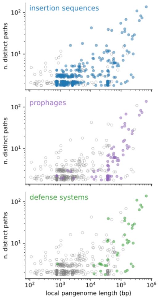
[15/N]
By looking at the content of the junctions, we find that the two peaks in binary junctions are explained by the movement of insertion sequences and prophages respectively, while hotspots are very flexible regions, rich in mobile genetic elements and defense systems.
By looking at the content of the junctions, we find that the two peaks in binary junctions are explained by the movement of insertion sequences and prophages respectively, while hotspots are very flexible regions, rich in mobile genetic elements and defense systems.
January 6, 2025 at 5:12 PM
[15/N]
By looking at the content of the junctions, we find that the two peaks in binary junctions are explained by the movement of insertion sequences and prophages respectively, while hotspots are very flexible regions, rich in mobile genetic elements and defense systems.
By looking at the content of the junctions, we find that the two peaks in binary junctions are explained by the movement of insertion sequences and prophages respectively, while hotspots are very flexible regions, rich in mobile genetic elements and defense systems.
[14/N]
On the other end of the spectrum we find hotspots, regions with tens to hundreds of different distinct paths, and a total accessory genome content of tens to hundreds of kbp in length.
On the other end of the spectrum we find hotspots, regions with tens to hundreds of different distinct paths, and a total accessory genome content of tens to hundreds of kbp in length.
January 6, 2025 at 5:12 PM
[14/N]
On the other end of the spectrum we find hotspots, regions with tens to hundreds of different distinct paths, and a total accessory genome content of tens to hundreds of kbp in length.
On the other end of the spectrum we find hotspots, regions with tens to hundreds of different distinct paths, and a total accessory genome content of tens to hundreds of kbp in length.
[13/N]
If we scatter-plot these two quantities for all of the 519 junctions in the dataset, we find that the majority are binary, i.e. they contain only two possible distinct paths, of which one is often empty. Their length distribution is bimodal, with a peak around 1 kbp and another around 30 kbp.
If we scatter-plot these two quantities for all of the 519 junctions in the dataset, we find that the majority are binary, i.e. they contain only two possible distinct paths, of which one is often empty. Their length distribution is bimodal, with a peak around 1 kbp and another around 30 kbp.

January 6, 2025 at 5:12 PM
[13/N]
If we scatter-plot these two quantities for all of the 519 junctions in the dataset, we find that the majority are binary, i.e. they contain only two possible distinct paths, of which one is often empty. Their length distribution is bimodal, with a peak around 1 kbp and another around 30 kbp.
If we scatter-plot these two quantities for all of the 519 junctions in the dataset, we find that the majority are binary, i.e. they contain only two possible distinct paths, of which one is often empty. Their length distribution is bimodal, with a peak around 1 kbp and another around 30 kbp.
[12/N]
We look at the local graph between two adjacent core blocks, that we call a junction graph. In this graph the diversity can be quantified in terms of number of distinct paths and total accessory sequence content.
We look at the local graph between two adjacent core blocks, that we call a junction graph. In this graph the diversity can be quantified in terms of number of distinct paths and total accessory sequence content.

January 6, 2025 at 5:12 PM
[12/N]
We look at the local graph between two adjacent core blocks, that we call a junction graph. In this graph the diversity can be quantified in terms of number of distinct paths and total accessory sequence content.
We look at the local graph between two adjacent core blocks, that we call a junction graph. In this graph the diversity can be quantified in terms of number of distinct paths and total accessory sequence content.
[11/N]
Next we investigate the structural diversity in the accessory genome. The fact that the order of core-genes is mostly conserved provides a well-defined frame of reference in which to study accessory variation.
Next we investigate the structural diversity in the accessory genome. The fact that the order of core-genes is mostly conserved provides a well-defined frame of reference in which to study accessory variation.
January 6, 2025 at 5:12 PM
[11/N]
Next we investigate the structural diversity in the accessory genome. The fact that the order of core-genes is mostly conserved provides a well-defined frame of reference in which to study accessory variation.
Next we investigate the structural diversity in the accessory genome. The fact that the order of core-genes is mostly conserved provides a well-defined frame of reference in which to study accessory variation.
[10/N]
However, the fact that synteny is largely conserved across big evolutionary distances, and the fact that many of these changes happen on terminal branches of the tree, indicate that these changes are likely removed by purifying selection.
However, the fact that synteny is largely conserved across big evolutionary distances, and the fact that many of these changes happen on terminal branches of the tree, indicate that these changes are likely removed by purifying selection.

January 6, 2025 at 5:12 PM
[10/N]
However, the fact that synteny is largely conserved across big evolutionary distances, and the fact that many of these changes happen on terminal branches of the tree, indicate that these changes are likely removed by purifying selection.
However, the fact that synteny is largely conserved across big evolutionary distances, and the fact that many of these changes happen on terminal branches of the tree, indicate that these changes are likely removed by purifying selection.